
SAVEPOINT ;
국제 FRM Part 2 오답·개념 정리 본문
Chapter 1
Market risk measurement and management
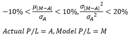
▶VaR Backtesting
Actual/Hypothetical return을 사용 (Hypothetical return → 다른 것들은 일정한 상태에서의 수익률)
짧은 기간을 사용해 오차 줄이기
|
Actual return
|
검증 실패 시 Intraday trading 문제
|
|
Hypothetical return
|
검증 실패 시 VaR 모델 수정 필요
|
|
Trading return
|
Actual return-Fee/Commision
|
|
Cleaned return
|
Actual return±Intraday trading
|
▶Correlation/Correlation volatility
|
Correlation
|
Stressed>Normal>Expansion
|
|
Correlation volatility
|
Normal>Stressed>Expansion
|
|
Types
|
Correlation
|
Correlation volatility
|
Reversion Rate
|
Distribution
|
|
Equity
|
35
|
80
|
78
|
Johnson SB
|
|
Bond
|
42
|
64
|
26
|
GEV
|
|
Default Probability
|
30
|
88
|
30
|
Johnson SB
|
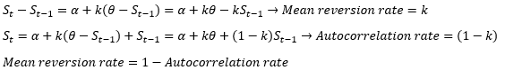
▶Mean reversion rate and autocorrelation rate
▶VaR backtesting
|
Unconditional coverage
|
Dependency, Timing 무시하고 단순히 Exception의 개수만 사용
|
|
Conditional coverage
|
Dependency (Clustered), Time variation 고려
|
▶Term-structure of Interest rate
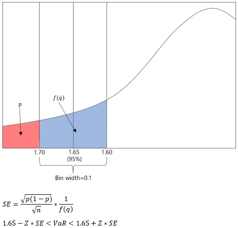
▶Backtesting Expected shortfall (95% 모델의 검증)
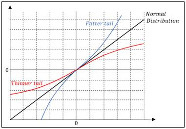
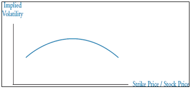
▶Volatility Smirk
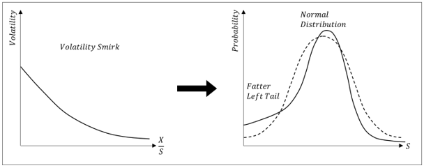
High Implied Volatility → Fatter tail than Log-normal distribution
▶Historical simulation methods
▶QQ plot
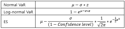
▶VaR and ES in normal distribution
▶Hill estimator – Consistent estimator for the Shape parameter ξ
1. Semi-parametric (Number of observations를 임의적으로 선택)
2. MLE (Maximum likelihood method) 사용
3. Consistency/Asymptotically normal (점근적 정규분포) 만족
▶Relationship of TypeⅠ/Ⅱ Error
TypeⅠ, TypeⅡ Error는 서로 Trade-off 관계
하지만, 표본의 수 n이 증가하면 TypeⅠ, TypeⅡ Error 모두 감소할 수 있음
▶Principal mapping
중간의 Coupon을 무시하고 만기 상환만 고려하므로 Duration을 크게 측정 → Overstates risk
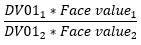
▶DV01 risk weights
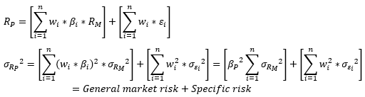
▶Variance of portfolio
▶Multi-asset options
대부분 Lower correlation → Higher option value
▶Correlation measures
|
Dynamic correlation
|
Deterministic/Stochastic approach
|
|
Static (Constant) correlation
|
Copula, VaR, Binomial
|
▶Concentration ratio and default correlation
대출의 Concentration ratio (1/Number of loans)가 감소하면 Joint default probability도 감소
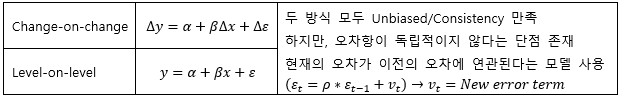
▶Regression hedge
It gives an estimate of the hedged portfolio’s volatility over time
Assumption of Constant β
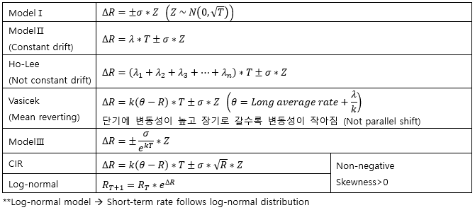
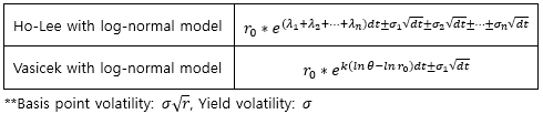
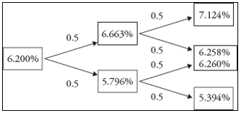
▶Log-normal model of Interest rate model
▶Time dependent Interest rate model
Useful for pricing interest rate Caps and Floors
▶Arbitrage-free Interest rate model
|
Arbitrage-free
(Ho-Lee model)
|
시장에서 관찰되는 가격이 맞는 가격이라고 가정
→ 시장 가격은 다양한 요인들에 의해 왜곡될 수 있음
On-the-run 증권의 가격을 이용해 Off-the-run 증권 가격 도출
→ On-the-run pricing이 틀릴 경우 Off-the-run pricing도 틀림
|
|
Equilibrium
(Vasicek model)
|
두 증권의 가치를 비교하는 Relative analysis에서는 Equilibrium 모델 사용
|
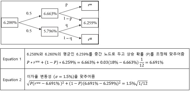
▶Not combining of vasicek model
Vasicek 모델은 평균 회귀 속성을 지니므로 중간 노드의 이자율이 달라지는 경우 발생
Combining 방법 (두 개의 방정식을 사용해 ruu, P 도출)
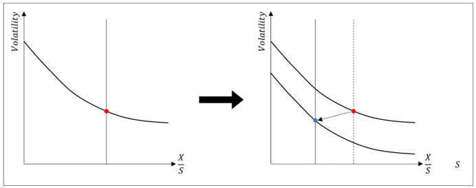
▶Implied volatility of equity option
|
내재변동성 곡선 위에서의 움직임
|
Stock price (S)↑ → X/S↓ → Implied volatility ↑ (+)
곡선 상에서 왼쪽으로 곡선을 올라타며 상승
|
|
내재변동성 곡선 자체의 움직임
|
Stock price (S)↑ → Implied volatility ↓ (-)
곡선 자체가 아래로 이동
|
곡선 자체의 이동 효과가 더 크기 때문에 종합적으로는 Stock price (S)↑ → Implied volatility ↓ (-) 관계
**Minimum variance delta: BSM Delta>Minimum variance delta
▶Vasicek interest rate model
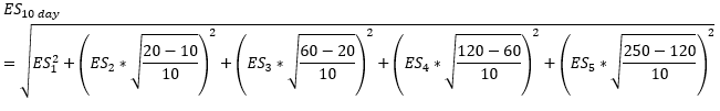
▶FRTB
1. ES
|
Category
|
Days
|
ES
|
Category 1
|
Category 2
|
Category 3
|
Category 4
|
Category 5
|
|
Category 1
|
10-days
|
ES 1
|
|
|
|
|
|
|
Category 2
|
20-days
|
ES 2
|
Fixed
|
|
|
|
|
|
Category 3
|
60-days
|
ES 3
|
Fixed
|
Fixed
|
|
|
|
|
Category 4
|
120-days
|
ES 4
|
Fixed
|
Fixed
|
Fixed
|
|
|
|
Category 5
|
250-days
|
ES 5
|
Fixed
|
Fixed
|
Fixed
|
Fixed
|
|
**각 ES는 Independent
2. Profit&Loss attribution
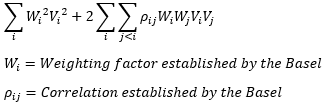
3. Revised standardized approach (상관관계를 고려하는 SA approach)
▶Volatility frown
Price jump → Volatility frown 형성
Chapter 2
Credit risk measurement and management
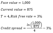
▶Credit spread
▶Fed funds/GC/Special rates
|
Fed funds – GC Spread
|
Fed funds rate-GC rate
위기에 국채 수요가 많아지며 GC rate 하락 → Spread 증가
|
|
Special Spread
|
GC rate-Special rate
|
▶Cap/Floor/Volatility of Special rate
|
Special rate
|
Floor
|
Cap
|
|
Before Global Financial Crisis
|
0%
|
GC rate
|
|
Penalty approach
|
0%
|
max(3%-GC rate, 0%)
|
Volatility of Special rate:
General collateral 보다 유동성이 높은 OTR 국채를 선호하므로 Auction 이전에는 Special spread가 크지만
Auction 이후에는 새로운 OTR 채권이 공급되며 가격이 하락 (Special rate 상승)
→ Special spread가 작아짐
▶Collateral Substitution/Rehypothecation/Segregation
|
Substitution
|
담보물을 자격이 있는 다른 것으로 대체
|
|
Rehypothecation
|
받은 담보를 제3자에게 담보로 사용
담보물 이동: X → Y → Z
Z 파산 시 Y는 X에게 담보물을 돌려줘야 하는 부채와 Z로부터 담보물을 받지 못한 손실을 감당
|
|
Segregation
|
Rehypothecation을 못 하도록 막는 조항
|
|
One-way CSA
|
두 상대방의 신용/규모에서 차이가 있는 경우
|
|
Two-way CSA
|
두 상대방의 신용/규모가 비슷한 경우
|
▶SPV Structure
Master trust structure: Frequent issues/Additional securitizations
▶PCA/PLS (Partial least squares)
|
PCA
|
PLS
|
|
Regression model
|
Regression model
|
|
Unsupervised
|
Supervised
|
|
변수 축소
|
변수 축소
|
|
Factor analysis (2nd Stage of PCA)
Rotation and varimax: 축을 회전시켜 Variance가 최대가 되도록 하는 주성분 선택
Canonial correlation method: Correlation이 최대가 되도록하는 Common dimension 도출
|
**PCA는 주성분들 중 Eigenvalue 값이 1보다 큰 것들만 사용
▶Single factor model
▶Mortgage securitized assets
|
Mortgage-backed bonds
|
자산을 Issuer의 Balance sheet에 남겨둠
|
|
REMICs
|
다양한 만기의 Class로 유동화 → 현금 흐름의 불확실성 완화
|
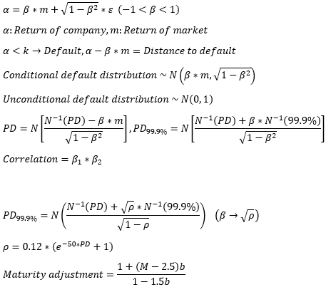
▶RWA
Off-balance 상품의 RWA는 CEA로 계산
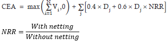
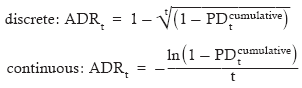
▶Annualized PD
▶Credit risks – Rating methodologies
|
Heuristic
|
Bottom-up, Expert-based, Qualitative, Low-cost, Human decision-making
Fuzzy logic: 어림/근사
익숙한 환경에서 많이 사용
|
||
|
Numerical
(통계적 접근)
|
Reduced form
|
Top-down
|
|
|
Neural
|
Top-down, 복잡/정돈되지 않은 Data에 사용, Non-linear
Black-box, Overfitting 위험
|
||
|
Structural
|
Merton model
|
||
|
Cash-flow modeling
|
Structural+Reduced form (Numerical) → Model risk가 중요
|
||
|
Clustering
|
Hierarchical
|
잎에서 뿌리로
|
|
|
Divisive
|
뿌리에서 잎으로
|
||
▶Correlated default time

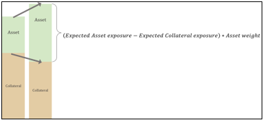
▶Collateral adjustment
1. Simple approach
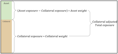
2. Comprehensive approach
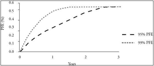
▶PFE
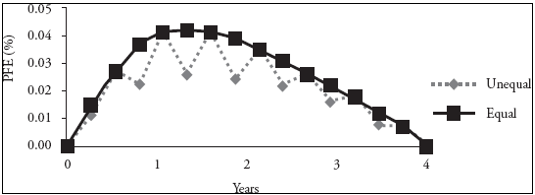
IRS에서 이자 지급/수취의 주기가 다른 경우
이자 수취의 주기가 더 짧다면 Exposure 감소 (위험 감소)
이자 지급의 주기가 더 짧다면 Exposure 증가 (위험 증가)
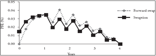
옵션은 행사일 이전에는 Exposure가 더 크고
행사일 이후에는 Exposure가 더 작아짐
CDS의 PFE는 LGD가 상한
▶CVA

▶BSM default model
회사 가치 (S)가 높을 때 주주 가치(주식, Call option)의 변동성이 작음
희사 가치 (S)가 낮을 때 주주 가치(주식, Call option)의 변동성이 큼
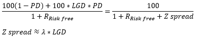
▶Risk-neutral Z-spread
▶RAROC
Operational risk 보다 Credit risk에 사용
Clawback/Deffered 등을 고려할 수 있는 Flexible method
▶Credit exposure
▶CDS/Credit-linked note
|
CDS
|
사건이 발생한 후 보험금을 받으므로 Counterparty risk가 큼
|
|
CLN
|
사건 발생 전부터 채권을 발행해 보험금을 선취하는 효과 → 채권 만기 동안 상환
보험금을 선취하므로 사건이 발생한 후에 보험금을 받지 못하는 Risk가 없음 (Counterparty risk 작음)
|
**Credit-linked note 매도 → CDS 매수와 비슷한 포지션
▶Merton model
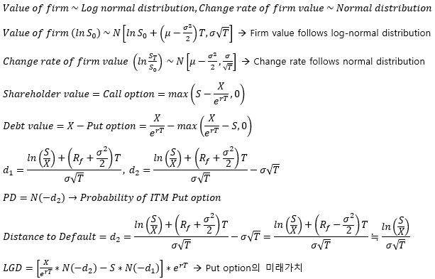
**Limitations
1. 비유동적/Non-public traded asset에 사용 불가
2. 변수들이 실시간으로 변하므로 끊임없이 계산되어야 함 (계산 비용 多)
3. 관측할 수 있는 변수여야 함
4. 갑작스러운 Default 반영 불가 (Jump-to-default)
5. Investment grade bond 보다 낮은 등급의 채권 평가에 적합
▶Defualt premium

▶Trade compressions
동일한 Reference asset을 지닌 거래 간 Netting (Multilateral)
▶Senior/Mezzanine/Equity Tranche
|
|
Senior
|
Equity
|
|
|
PD↑
|
Mean value
|
↓
|
↓
|
|
VaR
|
↑
|
↓
|
|
|
Correlation↑
|
Mean value
|
↓
|
↑
|
|
VaR
|
↑
|
↑
|
|
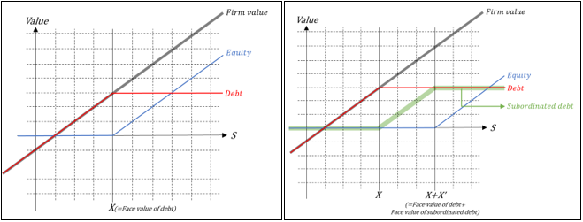
Mezzanine (≒Subordinated debt):
기업 가치가 높을 때에는 Senior (≒Debt)처럼 움직임
기업 가치가 낮을 때에는 Equity처럼 움직임
▶Interest rate dynamics and debt value
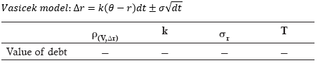
회사 가치와 이자율 변동의 관계 (ρ(V, Δr)가 클수록 Value of debt은 감소
나머지 요인들도 이자율의 변동성을 높이는 변수이므로 Value of debt과 (-) 관계
하지만, 이자율의 변동성이 높아질수록 Value of debt의 민감도는 작아짐 (체감적으로 감소)
▶Mortgage securitization frictions
|
Mortgagor (대출자) ↔ Originator (은행)
|
은행이 고객에게 부적합한 상품 추천
|
|
Originator ↔ Arranger (증권화의 주체)
|
Originator가 더 많은 정보 보유 (Adverse selection)
부실 자산을 넘겨줌 (Predatory Lending/Borrowing)
|
|
Arranger ↔ Third parties
|
Arranger가 더 많은 정보 보유 (Adverse selection)
|
|
Servicer ↔ Mortgagor
|
대출자는 자신의 재무 상태가 안 좋아지면 Servicer에게 지불해야할 금액들을 제대로 지불하지 않음 (Moral hazard) → Escrow 계좌를 통해 완화
|
|
Servicer ↔ Third parties
|
Servicer가 보수/비용을 과장 (Moral hazard)
|
|
Investor ↔ Rating agency
|
Investor는 정확한 등급 요구하지만 Rating agency에 비용을 지불하는 Arranger는 높은 등급을 원함 (Conflicts of interest)
투자자는 Rating agency의 Rating model을 모름 (Model risk)
|
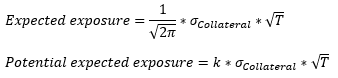
▶Potential expected exposure
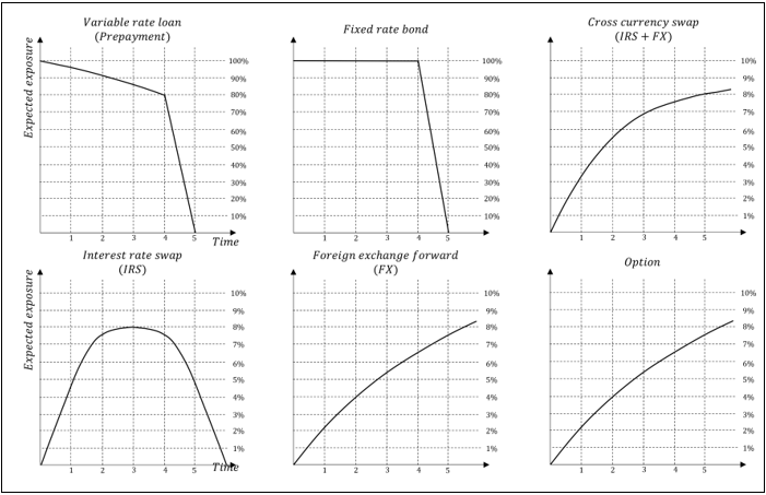
주기적으로 Payment 교환하는 상품 → Exposure가 커지다가 만기에 다가가며 축소 (닫힘)
만기에만 Payment가 존재하는 상품 → Exposure가 만기에 다가가며 계속 증가 (열림)
▶Netting factor
▶Netting
|
Payment netting
|
서로의 지불 금액을 Netting
MtM이 음수가 나오는 상품에서 Netting benefit 큼
Correlation이 클수록 Netting benefit 작아짐
|
||
|
Close-out netting
(특정 사건 발생)
|
Acceleration
|
지불 속도를 더 빠르게 함
|
상대의 부도 위험을 더욱 가속
(다른 투자자에게 위험 전가)
|
|
Close-out
|
현재 가치로 정산한 뒤 Out
|
||
|
Walk-away
|
상대 파산 시 MtM>0 이면 지불 요청, MtM<0 이면 지불 의무 없음
|
||
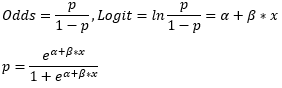
▶Logistic regression
▶Credit risk portfolio models
|
Credit Risk +
|
Credit Metrics
|
|
Independent Obligators의 Sensitivity 분석
Common factor, Only Default/Not default
|
Rating migration matrix (Joint migration)
→ 등급의 변화에 따른 가치 변화 반영
|
|
KMV
|
Credit Portfolio View
|
|
머튼 모형의 개량으로 복잡한 자본 구조도 반영
시장 환경의 변화를 빠르게 반영 가능
주식의 Correlation을 사용
|
거시 지표의 변화가 신용 위험에 주는 영향을 분석
|
**Limitations: Interest rates/Credit spreads/Current economic conditions 반영 불가
▶WWR (Wrong way risk) of Put option
OTM Put option이 ITM보다 WWR이 큼
▶Credit analysis comparison
|
|
Retail
|
Corporations
(Not financial)
|
Financial institutions
|
Sovereigns
|
|
Capacity
|
Wealth, Salary
Amount of debt
|
Cash flow from earning
Business strength
|
Liquidity
Asset quality
|
External debt
Tax receipts
Overall economy
|
|
Willingness
|
Reputation
Payment history
|
|
Sovereign ratings
Political environment
|
|
|
Evaluation
Methods
|
Credit scoring
|
Financial statesment
|
||
|
Loan size
|
Large size loans are secured → Mortgages
Small size loans are not secured → Credit loans
|
Larger size than retail loans
|
||
▶Audit report
|
Unqualified opinion
|
Meeting the minimum standards of presentation
|
|
Qualified opinion
|
Might not fairly represent the company’s financial situation
|
|
Adverse opinion
|
Not fairly represent the company’s financial situation
|
▶Good rating system
|
Objective&Homogeneity
|
Judgements based only on credit risk
Comparable among market segments, portfolio, customer types
|
|
Specificity
|
Measure DtD while ignoring other elements that are nor tied to default
|
|
Measurability&Verifiability
|
Correct estimation of default probability
Backtest rating model continuous basis
|
|
|
Rating agency
|
Internal expert
|
Heuristic
|
Numerical
|
|
Objective&Homogeneity
|
>
|
=
|
||
|
Specificity
|
>
|
<
|
||
|
Measurability&Verifiability
|
>
|
<
|
||
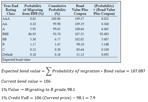
▶Credit VaR at CreditMetrics
▶Credit portfolio
▶Estimating PD
|
Risk-neutral
|
이론적으로 위험 중립이 될 때의 PD 사용
|
|
Historical
|
실제 Historical PD를 사용해 도출
|
▶Collateral management
|
Threshold
|
MtM>Threshold → 담보 설정
보호받지 못하는 금액
|
|
Initial margin
|
MtM과 무관하게 처음부터 보호되는 금액 (Independent amount)
Overcollateral
|
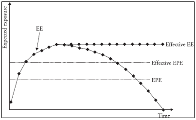
▶Expected exposure
▶MPoR (Margin period of risk)
담보 요청 후 실행까지 걸리는 시간
|
Valuation
|
담보물 밸류에이션
|
|
Receiving
|
담보물 수취
|
|
Settlement
|
담보물을 현금화 (증권의 경우 2-3일)
|
|
Grace period
|
유예기간
|
|
Liquidation/Close-out/Re-hedge
|
|
▶Credit spread curve and CVA

▶Incremental/Marginal CVA

▶Counterpary risk
|
Credit
|
Current exposure, Expected exposure 사용
|
|
Market
|
CVA, VaR of CVA 사용
|
▶WWR modeling
|
Hazard rate approach
|
Easy way but underestimation of WWR
Stochastic process for credit spreads
|
|
Structural approach
|
Easier than Hazard rate approach
Default/Exposure distributions mapped to Bivariate distribution
Early default time and Higher exposure → WWR
High correlation → High WWR
이미 존재하는 분포를 사용 (장점이자 단점)
|
|
Parametric approach
|
가장 직접적인 방법 (Direct approach)
Credit spread/Exposure의 Historical link 찾기
|
|
Jump approach
|
Most applicable to WWR (Implies a jump at default)
Jump factor=residual value(RV)
기초 자산 가격이 (1-RV)만큼 빠르게 하락
|
▶Example of WWR
1. Default of Lehman
리만브라더스 파산 후 일본 엔화 평가 절상
미-일본 달러 스왑에서 엔화를 담보로 더 많은 달러를 받을 수 있으므로 거래의 가치는 상승
하지만, 미국의 신용도가 악화됨
2. 경기 침체 시 이자율 하락
고정 금리 수취/변동 금리 지급 거래의 경우 이자율이 하락하면 거래의 가치는 상승
하지만, 경기 침체로 PD 상승함
3. Foreign currency transaction
자국 통화를 수취/Local 통화를 지급하는 거래의 경우 Local 국가의 경제 악화로 Local 통화가 평가 절하되면 거래의 가치는 상승하지만 상대 국가의 경제 악화로 신용도 하락
▶CVA
1. Exposure가 변동적인 상품에 적용 (Loan은 Exposure가 고정적 → CVA보다는 EAD 사용)
2. Aggregating CVA is not useful
CVA를 단순히 합한 것은 모든 상품이 동시에 Default된다는 가정이므로 비현실적
▶Credit scoring
|
Credit bureau scores (신용점수)
|
FICO score (300-850 score), Fast, Cost effective
|
|
Pooled model
|
Built by outside parties, Flexible to tailor it to a specific industry
|
|
Custom model
|
Lender’s own credit application pool
|
**Data characteristic: 데이터 분류/Attribute: 데이터 분류의 값들
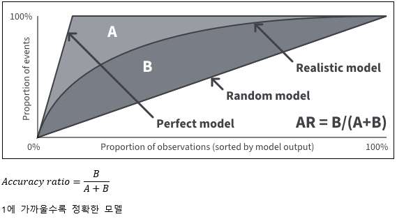
▶CAP
▶CDS 지급 방식
|
손해분 모두 보상
|
Face value-Current price
|
|
액면의 일정 % 보상
|
Face value*X%
|
|
액면 모두 보상 후 기초 자산 이전
|
|
▶Increasing prepayment speed
|
Interest rate ↓
|
Prepayment speed ↑
|
|
House price ↑
|
Prepayment speed ↑
|
|
Mortgage size ↑
|
Prepayment speed ↑
|
|
만기 ↓
|
Prepayment speed ↑
|
|
Default ↑
|
Prepayment speed ↑
|
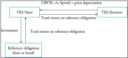
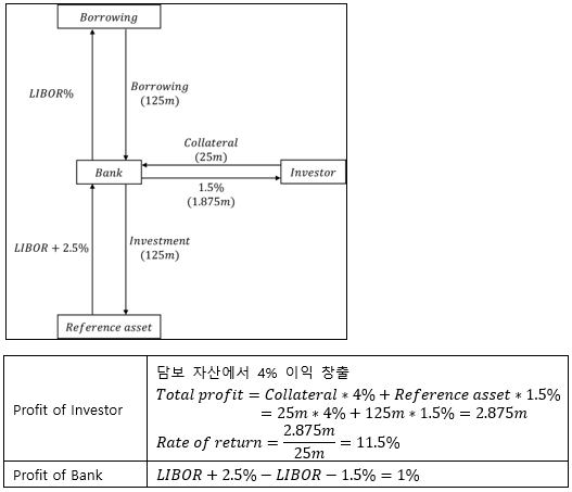
▶TRS/Asset-backed credit-linked notes
1. TRS
2. Asset-backed credit-linked notes (Asset-backed CLN)
▶Synthetic CDO/Single-tranche CDO
|
Synthetic CDO
|
자산을 넘기지 않고 CDS로 위험만 이전
|
|
Single-tranche CDO
|
특정 기초 자산을 선택 Customizable → Better spread
|
▶Auto loan ABS/Credit card/MBS/Student loans performance measures
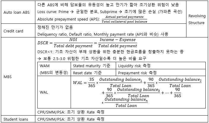
**Revolving structure
1. 짧은 만기/높은 조기 상환율의 상품에 많이 사용
2. Lump-sum (Not amortized)
3. Not pass-through → Buy new assets
▶ABS 신용보강
|
Excess spread
|
Cost of Assets > Cost of Liabilities → Administration expense 이후 남는 것 Reserve에 보유
|
|
Margin step-up
|
Call date 이후 Coupon 증가 (Inverstor에게 이익)
Call date 이후 발행자의 Call option 시작 (Issuer에게 이익)
|
|
Shifting interest
(Senior 신용 보강)
|
일정 기간/일정 금액까지 Senior에는 원금과 이자 지급, Mezzanine에는 이자만 지급
|
Chapter 3
Operational and integrated risk management
▶Operational risk management의 특징
|
Hard to centralize
|
각 Business unit에서 예방되어야 함
|
|
Dynamic
|
Difficult to Model/Quantify → Reactive가 중요
|
|
Heterogenous
|
같은 운영 리스크 내에서도 차이 多
|
|
Idiosyncratic
|
다른 리스크 유형과의 차이 多
|
▶Indirect/Non-financial operational risk impact
|
Indirect
|
Compliance, Reputation, Customer detriment
|
|
Non-financial
|
Customers, Employees, Third parties, Shareholders
|
▶Operational risk triggers
|
Reputation
|
명성 피해
|
|
Resilience
|
Goods/Service 문제
|
|
Materiality
|
Threshold를 초과한 Loss
|
|
Stability
|
재무 안정성 문제
|
▶RCSA
|
특징
|
Non-quantitative (Qualitative)
Preventive/Corrective
Prioritize risks, 설문 조사 형식 자주 사용
|
|
Inherent risk
|
Risk control 이전의 Gross risk
|
|
Residual risk
|
Risk control 이후의 Net risk
|
|
|
|
▶Line of defense
|
1st Line (Risk Owner)
|
Risk Measure/Manage/Oversight, Risk appetite 고려
Assessment of risks and control
|
|
1.5st Line (Risk Champion/Risk Specialist)
|
Spokeperson, Included in 1st Line
|
|
2nd Line
|
Oversight/Question, On-going monitoring
Deeper dives into specific risk
|
**회사 규모가 작은 경우 1st, 2nd Line이 통합될 수 있지만 독립성은 유지되어야 함
▶Backtesting
Likelihood는 과소평가
Impact는 과대평가
▶Operational risks taxonomy
|
Category
|
Severity
|
Frequency
|
|
Internal Fraud
|
Low
|
Low
|
|
External Fraud
|
Low
|
High
|
|
Employment&Workplace safety
|
Low
|
Moderate
|
|
Physical damage
|
Low
|
Low
|
|
System failures
|
Low
|
Low
|
|
Clients, products (1st Loss severity)
|
High
|
High
|
|
Execution, delivery
|
High
|
High
|
▶Operational risk assessment methods
|
Casual analysis
|
Future-orient, Not rely on historical data
|
Not one main cause
|
|
Fault tree analysis
|
Reverse scenario, Deductive
|
|
|
Factor analysis
|
각 Factor의 분포 추정 후 Monte-carlo 수행
|
|
|
Root-cause analysis
|
다양한 Cause&Impact 분석, 1st Line에서 수행
Bow tie diagram/5-Why analysis
|
|
|
Fixed multipliers
|
각 요인을 Multiply하여 극단적 손실 분석 → Dependency 반영 불가
|
|
|
LDA
|
손실 빈도/심각도의 독립적 분포 가정 → Economic capital 도출
높은 Skewness 반영 불가 → EVT로 보완 필요
|
One main cause
|
|
EVT
|
손실 분포의 High Skewness Tail 모델링
|
▶ Third party risk management (TPRM)
|
Business model decision
|
어떤 부문을 Out-sourcing할 것인지 선택
|
|
Due diligence/Evaluation/Risk rating
|
실사, 평가
|
|
Contracts
|
계약, 문서화
|
|
Monitoring
|
|
|
Termination/Remediation
|
Intellectual property의 계약 종료 후 소유권 정리/이전
→ 성공/실패의 성과 수준을 결정 (Performance metrics)
|
**Business continuity/Contigency plans are important for outsourcing risks
▶Solvency Ⅱ
|
Regulatory capital
|
SA/IRB (99.5%, 1-Year) approach
|
|
Risks
|
Underwriting/Investment (Market, Credit)/Operational risk
|
▶Scenario analysis workshop
Seniors of each Business units, Risk specialist로 구성
1. Silent voting: Dominant personalities의 문제를 완화
2. Common assessment bias: Excess focus on scenarios driven by external causes
▶Risk reporting cake
|
Tier 1
|
Daily Reporting/Monitoring
|
|
Tier 2
|
Action → 부족한 점을 수정/위험 완화
|
|
Tier 3
|
Decision-making
|
▶Qualitative risk data aggregation
|
Conversion&Addition
|
Qualitative risk를 Monetary unit으로 전환 (Additive, Linear)
|
|
Categorization
|
Graphical format (Heat-map approach)
|
|
Worst-case reporting
|
그룹 중 가장 최악의 Case를 기준으로 전체 그룹 결정 → Most conservative
|
▶Input/Processing/Reporting
|
Input
|
→
|
Processing
|
→
|
Reporting
|
|
Data 입력치
|
Estimation 도출
|
Converting estimation to useful report
|
|
Model risk
|
Down-side만 존재
대상 모델과 연관된 다른 모델도 검증해야 함
|
|
Execution risk
|
잘못된 Input data/Coding
|
|
Conceptual errors
|
잘못된 모델 가정/모델링
→ Gaussian constant: CDO 상품에 대한 잘못된 위험 평가로 금융 위기 발발 요인 제공
(정상적 상황을 가정해 Low Correlation/Constant relationship 가정)
|
▶Diversification impact methods
|
Stand-alone
|
분산효과 무시
|
|
Fully diversified capital
|
분산효과를 각 크기 비율로 분배
|
|
Marginal capital
|
새로운 자산/활동이 추가될 때 증가하는 요구자본
|
▶SA approach
10년 데이터 필요 부족할 경우 5년 데이터 사용
데이터가 너무 부족한 경우 BI만을 SA로 사용
▶Risk 인식 과정
|
Occurrence
|
Discovery
|
Reporting
|
Accounting
|
|
|
Visibility
|
Timeliness
|
|
||
▶Heat map
|
Extreme
|
Amber
|
Red
|
|
|
|
|
Very high
|
Yellow
|
Amber
|
Red
|
|
|
|
High
|
Green
|
Yellow
|
Amber
|
Red
|
|
|
Medium
|
|
Green
|
Yellow
|
Amber
|
Red
|
|
Low
|
|
|
Green
|
Yellow
|
Amber
|
|
|
Remote
|
Unlikely
|
Possible
|
Likely
|
Highly
Likely
|
▶ Human errors
|
Not Intentional
|
Slips
|
Fat finger, Skill based errors
|
|
Intentional
|
Rule based
|
잘못된 체계 등으로 인한 이해상충/에러
|
|
Knowledge based
|
교육, 보조 자원의 부족으로 인한 에러
|
|
PDSA – Quality improvement
|
Lean-six sigma
|
Prevent through design
|
|
|
Plan
|
Setting goal, Make process
|
Lean:
Eliminating waste
Six sigma:
Minimizing variability
|
Optimizing processes by creating checklists, protocols, systems
|
|
Do
|
Execution, Collect data
|
||
|
Study
|
Analysis data → Find improvement point
|
||
|
Act
|
Making adjustment
|
||
▶VaR multiplier
|
Backtesting exceptions
|
Multiplier
|
|
5개 미만
|
3.0
|
|
5 / 6 / 7 / 8 / 9
|
3.4 / 3.5 / 3.65 / 3.75 / 3.85
|
|
10개 초과
|
4.0
|
▶Investor protection
|
MiFID Ⅱ
|
글로벌 금융 위기 이후
Public disclosure for trading data
Best execution
Interest conflicts
|
|
Dodd-Frank
|
내부고발자 보호
OTC 규제
Clearing house 사용 요구
|
|
Volcker rule
|
자기 자본 투자 규제
|
▶Business Continuity/Resilience
|
Contigency Planning
|
Business Continuity
|
Recover each business in timely basis
|
|
Resilience
(Disaster recovery)
|
Recover important business problem under Impact tolerance
Impact tolerance를 초과하는 경우는 다루지 않음
Resource allocation을 통해 Impact tolerance가 Branch되지 않도록함
|
▶Combine internal/external operational loss data
Internal loss data는 High-frequency/Moderate-severity에 집중되어 있음 → External loss data 이용해 보완
1. Scaling: External loss data를 Scaling하여 사용
2. Cut-off mix: Threshold 이후 부족한 Data를 External data를 포함해 분포 추정
3. Filtering: 데이터 포함/제외 기준 설정
▶Risk identification
|
Top-Down approach
|
|
|
Exposure
|
Major client, Key revenue source
|
|
Vulnerabilities
|
Weak points, Control weakness
|
|
Risk wheel
|
Deeper understanding of causes/effects
|
|
Unexpected risk
|
Horizon scanning
|
|
Bottom-Up approach
|
|
|
Loss data analysis
|
Internal/External/Near miss
|
|
RCSA
|
Performed by 2nd Line, Qualitative, Prioritize risks
|
|
Process mapping
|
Stating individual steps
Find potential problems
|
▶New initiative risk assessment process (NIRAP)
|
Objective
|
새로운 상품 도입 이유
|
|
Alternative
|
다른 대안
|
|
Expected benefits/disadvantages
|
기대 효과
|
|
Commercial aspect
|
Funding needs and Cost
|
|
Risk&Mitigants methods
|
리스크와 완화 조치
|
|
Initial stage
|
Risk identify/assess, Plan for risk mitigation/monitoring
|
|
Project life
|
Regular reporting
|
|
Project closure
|
Evaluation, Debriefs, Lesson learned
|
▶Contigency planning
|
Speed
|
Timely basis
|
|
Competence
|
Should be assigned to risk management specialists
|
|
Transparency
|
현재 상황을 이해 관계자들에게 Disclosure
|
|
Recovery Point Objective (RPO)
|
어느 수준까지 회복해야하나
|
|
Recovery Time Objective (RTO)
|
언제까지 회사가 버틸 수 있나
|
▶ Business indicator
|
BI
|
Weight
|
|
|
~1B
|
Bucket1
|
12%
(BIC에 ILM을 곱하지 않음)
|
|
1B~30B
|
Bucket2
|
15%
|
|
30B~
|
Bucket3
|
18%
|

▶Stresstesting
|
Quantitative
|
Parameter stress test
|
|
Qualitative
|
Reverse stress test
|
|
Quantitative&Qualitative
|
Macroeconomic stress test (Regulator 제공)
|
|
Legal loss add-on
|
법적 Loss 반영
Event 발생과 Loss의 시기가 달라 어려움 존재
|
|
Idiosyncratic add-on
|
각 은행의 개별적인 위험 반영
|
**Stresstest는 Coherence가 중요
▶Financial Crime/Fraud
|
Internal fraud
|
Unauthorized activities, theft and fraud
Selection (정직한 직원 고용), Prevention (업무의 분리), Detection
|
|
External fraud
|
System security, theft and fraud
First-party fraud: 고객/파트너의 사기
|
▶Cyber security
|
Regulator가 Requirements 직접 제시
|
Emerging market에서 많이 사용
Sector-specific: Homogeneous banking system에 적합
Cross-sectoral: Fragmented banking system에 적합
|
|
각 은행/기관이 자신들의 IT전략 제시
|
Europe/선진국에서 사용
|
|
NIST CSF
|
미국에서 Critical Infrastructure을 지키기 위해 시작
|
|
ISO 27001
|
Key global standards
|
|
CIS
|
NIST, ISO를 보완
|
**CIA: Confidentiality, Integrity, Availability (Business continuity)
|
Information control
|
|
|
Behavioral
|
Human error
|
|
Technical
|
Preventative (방화벽, 암호화), Detective (Early warning), Mitigation (Backup)
|
▶AML risk
|
Placement
|
불법 자금을 Smurfing (큰 금액을 작은 금액으로 여러 번 거래)하여 배치시킴
|
|
Layering
|
Multiple account로 복잡한 거래를 통해 세탁
|
|
Integration
|
자산 거래 등으로 불법 자금을 Economy에 결합
|
|
AML Risk management
|
|
|
Selection
|
KYC, Due diligence (Sanctions list)
|
|
Deterrent
|
계좌 정지, 고소
|
▶Third party risk
|
계약 관련 조항
|
||
|
Indemnification (면책)
|
3rd Party에 의한 문제를 고용 기관이 책임지지 않을 수 있음
|
|
|
Subcontracting (재하청)
|
Primary 3rd Party가 Subcontract의 책임을 짐
|
|
|
Right to audit
|
Optional 조항
|
|
|
Limit liabilities
|
||
|
Foreign-based service
|
혼동을 줄이기 위해 하나의 관할 지역의 법/조항 적용
|
|
▶ Economic capital

|
Strategic capital
|
|
|
Good will
|
Purchase price > Fair price
|
|
Burned-out capital
|
Start-up에 투자한 금액 → 시간이 지날수록 감가되어 감
|
|
Economic capital Constraints/Opportunities
|
||
|
Types
|
Constraints (-)
|
Opportunities (+)
|
|
Credit portfolio management
|
각 고객의 신용도를 판단하지 않음
|
Appropriate hedging strategies
Protect risk deterioration
|
|
Risk-based pricing
|
|
Maximize bank’s profitability
|
|
Customer profitability analysis
|
Difficult to measure
|
더 높은 수익률의 고객에 Economic capital 할당 가능
|
|
Management incentives
|
Compensation에 RAROC를 사용하는 것은 제한적
|
|
▶Model validation
|
Qualitative
|
|
|
Examination of assumptions
|
|
|
Qualitative review
|
|
|
Quantitative
|
|
|
Input/Parameter validation
|
|
|
Model replication
|
Same output을 만든다고 적합한 모델은 아님 → Little evidence
|
|
Benchmarking
|
Standard model과의 적합성만 비교 → Little comfort
|
|
Backtesting
|
Output과 Forecast를 비교
|
**Normal/Stressed 상황 모두에서 검증해야함
|
|
Qualitative
|
Quantitative
|
|
Conceptual soundness
|
Sensitivity analysis
|
|
|
Ongoing monitoring
|
|
Benchmarking
|
|
Outcome analysis
|
Expert judgement
|
Backtesting
Parallel outcomes analysis (기존 모델과 새로운 모델 비교)
|
|
Third-party models
|
Hard to validate
Some parts of the modeling may be confidential
|
|
▶BHC (Bank holding company)
|
Risk identification
|
가능한 모든 Risk 식별
(Normal/Stress, Changing environment, On/Off balancesheet)
|
|
Internal controls
|
Audit team carefully scrutinize internal control, Documentaion
|
|
Governance
|
Board는 Senior manger의 자료를 바탕으로 의사결정
|
|
Capital policy
|
Dividend, Repurchase, Contigency plan
|
|
Stresstesting
|
은행의 Unique 특성 반영, Not optimistic → Conservative approach
|
|
Estimating Loss/Revenue/Expense
|
Not constant relaitonship → Sensitivity analysis 필요 (보수적 가정)
Automated system → 수동적 개입 방지
Stressed 상황에서는 Long-run average 사용 금지
|
▶Foundation/Advanced IRB
|
Foundation IRB
|
담보 효과는 Comprehensive approach 사용
PD≥0.03%, LGD=45% (Senior)/75% (후순위), M=2.5
|
|
Advanced IRB
|
Bank’s own estimate
PD≥0.03%
|
|
Retail
|
Bank’s own estimate
No Maturity adjustment (MA)
|
▶Incremental risk charge/Comprehensive risk charge
자본요구를 줄이기 위해 자산을 Banking book (자본 요구 기준: 99.9% 1-Year)에서 Trading book (자본 요구 기준: 99%, 10-Day)으로 옮기는 은행들이 많았음
|
IDRC
(Incremental default risk charge)
|
Trading book의 자산도 Default-sensitive하면 99.9%, 1-Year를 적용하도록 함
→ Down-grade risk를 반영하지 못함
|
|
IRC
(Incremental risk charge)
|
Default-sensitive에서 Credit-sensitive 자산까지 확장
Liquidity horizon 안에 등급이 하락하면 해당 자산을 매도하고 동일한 등급의 자산으로 교체
→ Credit spread risk, Expected shortfall로 측정
→ Jump-to-default risk: 높은 신뢰도의 VaR로 측정
|
|
Comprehensive risk charge
|
Correlation-sensitive 자산의 경우 추가적 자본 요구
|
**Trading book 분류 요건:
1. 물리적으로 거래 가능한 자산
2. 해당 자산의 리스크가 Trading desk에서 관리됨
▶Positive feedback traders
|
Stop loss
|
가격 내리면 매도 → Destabilize
|
Positive feedback
|
|
Short Call/Put
|
가격 내리면 매도 → Destabilize
가격 오르면 매수 → Destabilize
|
|
|
Portfolio insurance
|
주가 오르면 주식 매수 → Destabilize
주가 내리면 주식 매도 → Destabilize
|
|
|
Dynamic hedge
|
Negative feedback → Stabilize
|
Negative feedback
|
▶Future hedge/Option hedge
|
Future
|
일일 정산/마진 콜 등으로 Liquidity risk 존재
|
|
Long option
|
초기 프리미엄 지불 후에는 추가적 자금 불필요, Liquidity risk 완화
|
▶Stresstesting programs
|
Pre-SCAP
|
미시적/Static/Single-shock scenario
Focus to Earnings
|
||
|
SCAP
|
거시적/Dynamic/Macro-scenario (One-size-fits-all)
Firm-wide (Both bank level and asset class level)
Focus to Capital requirement, Revenue and Cost
→ 당시 은행들의 자본 적정성 향상에 기여
|
||
|
CCAR
|
2011
|
Macro/Bank specific scenario → Macro-scenario 결과만 Public disclose
|
Stresstest Only
|
|
2012
|
Macro/Bank specific 결과 모두 Public disclose
|
||
|
EBA
|
은행 추정치와 Third-party 추정치 비교
테스트 결과를 웹을 통해 다운로드 가능 (Disclosure 향상)
More detailed (Geographical, Regions, Asset class)
Both Stress/Base test
|
||
▶Anti ML/FT
|
1st Line
|
Screening potential employees
|
|
Monitoring
|
All transactions
|
|
Customer due dilligence
|
위험도 높은 인물 위주로 검사 (큰 액수, 잦은 해외 거래, 블랙리스트)
|
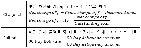
▶Charge-off/Roll-rate
▶Operational risk reports
|
Decision-makers
|
간단하고 Firm-wide한 지표들 필요 → Decision-making에 용이
|
|
Each business managers
|
더 상세한 지표들 필요
|
|
Backward-looking indicators
|
Backward-looking 지표들도 필요함
|
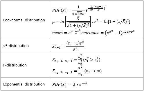
▶Log-normal distribution/X2-distribution/F-distribution/Exponential distribution
▶Use of Point-in-time/Through-the-cycle
|
Point-in-time
|
Pricing, Credit exposure, Short-term (변동적인 요소들)
|
|
Through-the-cycle
|
Strategy decision, Economic capital, Long-term (변동적이지 않은 요소들)
|
▶Risk management failures case study
|
Liquidity crisis
|
|
|
Lehman
|
단기 차입으로 비유동적 장기 자산 투자 (CDO)
|
|
Continental Illinois
|
Oil&Gas Market player, 높은 금리로 단기 자금 조달 실패
|
|
Nothern Rock
|
OTD Business Bank
|
|
Ashanti goldfields
|
Sold gold forwards, 급격한 가격 상승으로 마진 콜
|
|
Hedging crisis
|
|
|
Metallgesellschaft
|
장기공급계약 (Short)을 단기 선물 (Long)으로 롤링 헤지
마진 콜 발생 후 유동성 부족
|
|
Model risk crisis
|
|
|
Niederhoffer
|
Deep OTM Put 판매 → 극단적 상황 발생 (1일 7% 하락)
모델에서는 거의 불가능한 확률이 발생함
|
|
LTCM
|
비유동 국채 매수, 유동 국채 매도 전략 → 스프레드가 오히려 커지며 손실
|
|
London whale
|
VaR Limit을 조작
|
|
Barclay’s
|
엑셀 Spread sheet 사용으로 잘못된 거래 수행
|
|
Rogue trading crisis
|
|
|
Barings Bank
|
Leeson이 회사 지시를 무시한 채 방향성 투기, 회계 조작
|
|
Reputation risk crisis
|
|
|
Volkswagen
|
테스트에서만 이산화탄소 저감 장치 장착
|
|
Governance crisis
|
|
|
Enron
|
부정 회계, 감사 실패
|
|
잘못된 금융공학 상품 사용
|
|
|
Bankers Trust
|
이자율 파생 상품
|
|
Orange County
|
FRN 상품
|
|
Sachsen Landes Bank
|
Subprime 증권화 상품 투자
|
|
Cyber security crisis
|
|
|
Equifax
|
IT System의 List 부재, 만료된 증명서, Poor internal/external communication
3개월간 데이터의 유출을 인지하지 못함 (Low visibility)
|
|
Anti ML/FT
|
|
|
USAA
|
실제 사건이 발생하지는 않았지만 부적합한 시스템으로 벌금 부과
|
|
Third-party risk
|
|
|
Capital one
|
Amazon AWS의 전 직원이 시스템의 취약점을 이용
|
|
Morgan Stanley
|
3rd Party에게 위탁한 Decommissioned hardware가 여전히 기밀 정보를 가지고 있었음
|
|
Investor protection
|
|
|
UBS
|
잘못된 상품 설명
|
|
JP Morgan
|
거래량 조작 (Spoofing) → 회사에 이익이 되도록
|
|
Deutsche Bank
|
Rebate를 얻으며 고객의 최대 이익에 부합하지 않게 영업 활동 → Best execution 위반
|
▶Key indicators
|
Key risk indicators
|
직원 당 거래 횟수, 인센티브 기준 판매 목표치 증가
|
|
Key performance indicators
|
고객 컴플레인 횟수, Error rate
|
|
Key control indicators
|
Business continuity plan의 업데이트/리뷰 횟수, 리뷰 이후에 발생한 에러 횟수
|
▶Due diligence Third-party
|
Business background, reputation, strategy
|
History, Business model
|
|
Financial performance and condition
|
Financial stability, Insurance coverage
|
|
Operations and internal controls
|
Internal controls, IT systems, Staff training
|
▶벌금 산정의 고려 사항
1. Deter other firms against manipulative bank practices
2. Ensure that fines cover at least the benefits of breaches
3. Signal to other firms to change their compliance practices
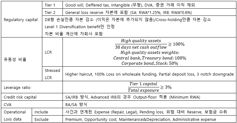
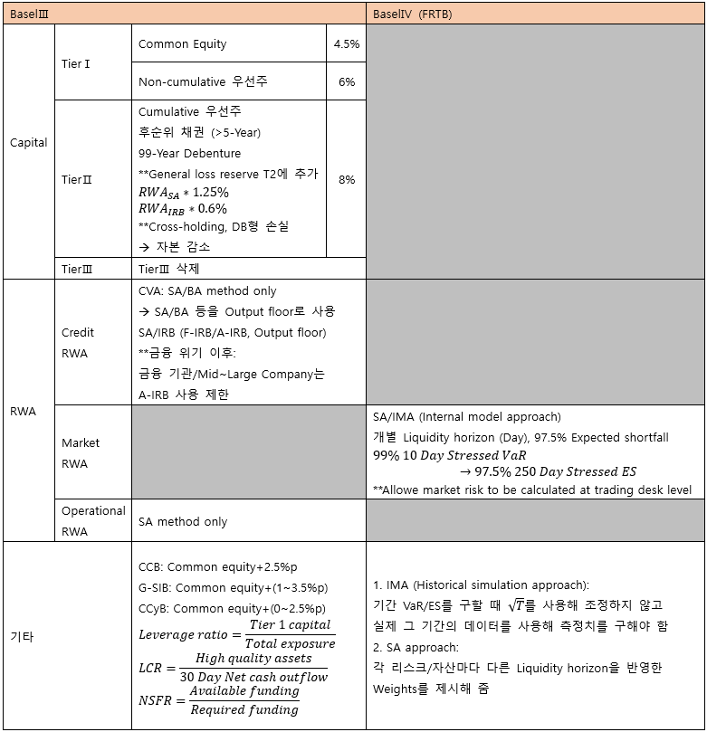
▶Basel Ⅲ
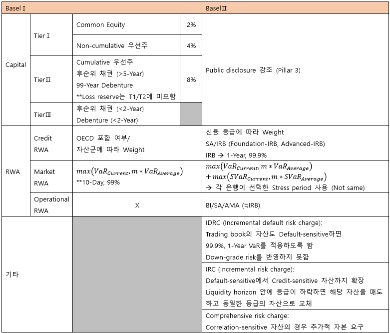
▶BaselⅠ/Ⅱ/Ⅲ/FRTB
▶Risk measures
|
Methods
|
Coherence
|
Stability
|
특징
|
|
Standard deviation
|
Not Monotonicity
|
Not Stable
|
|
|
VaR
|
Not Subadditivity
(Normal distribution에서는 만족)
|
Not Stable
|
Absolute risk measure
Capital allocation
|
|
ES
|
Coherent
|
May or may not stable
|
Capital allocation
|
|
Spectral/Distorted
Risk measures
|
|
May or may not stable
|
직관적이지 않음
이해하기 어려움
|
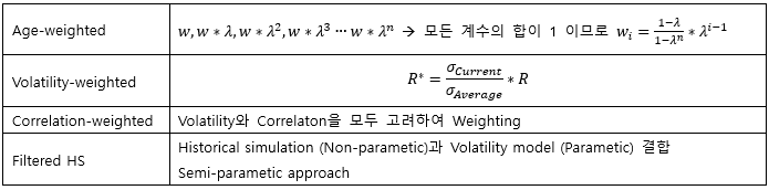
▶Risk aggregation methods
|
Simple summation
|
분산 효과를 무시하고 단순히 합함
|
|
Constant diversification
|
Simple summation에서 일정 %를 분산 효과로 감소시킴
|
|
Variance-covariance matrix
|
모든 Variance/Covariance 고려하여 분산 효과 반영
많은 계산, Non-linear/Skewness 고려하지 못함
|
|
Copulas
|
Parametric method로 Joint distribution 도출
|
|
Full modeling/Simulation
|
Non-parametric (Simulation) method로 Joint distribution 도출
|
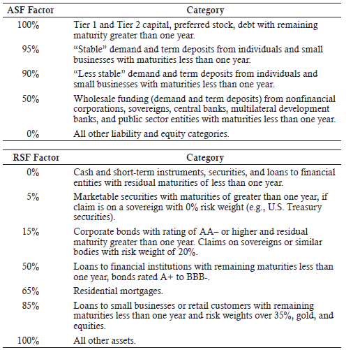
▶ NSFR
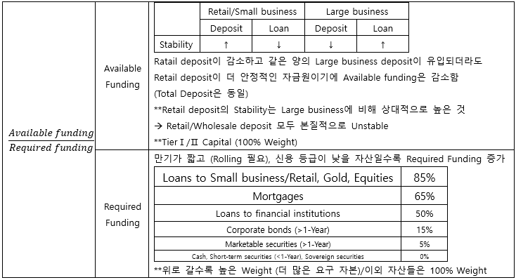
▶NSFR Weights details
Chapter 4
Liquidity and treasury risk measurement and management
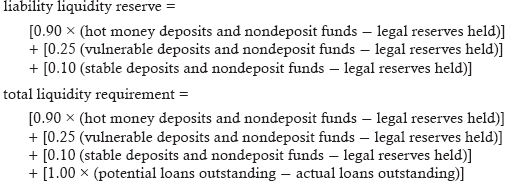
▶Available funding gap
유형 자산 매각/매수, 사업비/운영비는 제외

▶MMF valuation
매우 짧은 만기로 이자율/스프레드의 영향이 미미하기에 시가 평가를 하지 않음
1 Share=$1.00 → NAV가 $1.00 아래로 내려갈 수 있음 (Breaking the buck)
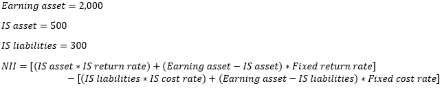
▶NII Calculation
▶Liquidity needs
|
Types
|
Stability
|
|
Core deposit (Stable deposit)
|
↑
|
|
Vulnerable
|
-
|
|
Hot money
|
↓
|
▶Non-deposit liabilities
|
Types
|
특징
|
Size
|
Stability
|
Cost
|
||
|
Fed funds
|
Overnight:
다음날에 상환
Term:
Few Days, Weeks, Months
Continuing:
한 쪽이 거래를 중지하기 전까지 만기 연장
|
Large/Small
|
Volatile
|
High
|
||
|
Discount window
|
Primary/Secondary:
신용도 차이
Seasonal:
Long-term, 가장 낮은 이자율
|
|
Low
(담보 설정)
|
|||
|
CDs
(3개월)
|
Dollar-Denominated CDs
(Euro CD)
|
해외에서 USD로 CD 발행
|
Large
|
Stable
|
High
|
|
|
Yankee CDs
|
외국인이 미국 지점에서 CD 발행
|
|||||
|
Thrift CDs
|
비은행 발행
|
|||||
|
Eurocurrency (3개월)
|
3개월 이내
|
|
||||
|
CP (270일)
|
최대 270일
|
Stable
|
||||
|
Banker’s acceptance (6개월)
|
수출/수입 관련
|
|
||||
|
Municipal bonds
|
Tax-Anticipated
|
지방 정부 세금 수입으로 지급
|
|
Revenue-Anticipated 보다 안정적
|
|
|
|
Revenue-Anticipated
|
특정 프로젝트로 수익 지급
|
|
||||
**Non-deposit liabilities → Interest sensitive, Flexibility
▶Liquidity types
|
Operational
|
Day-to-Day operation liquidity
|
|
Contigent
|
Liquidity asset buffer for stress time
|
|
Strategic
|
자산 매입, 투자를 위한 유동성
|
|
Restricted
|
담보로 이용된 자산 → 활용성 낮음
|
▶Commercial vs Retail loan risk
|
Commercial loan
|
Retail loan
|
|
Large size/Few loans → Extreme risk
Not enough diversification
|
Small size/Many loans → Predictable (Cost로 인식)
Enough diversification, Early warning signal 사용 가능
|
|
Semi-automated loan system → System risk 발생 가능
새로운 상품의 경우 Historical data 부족
|
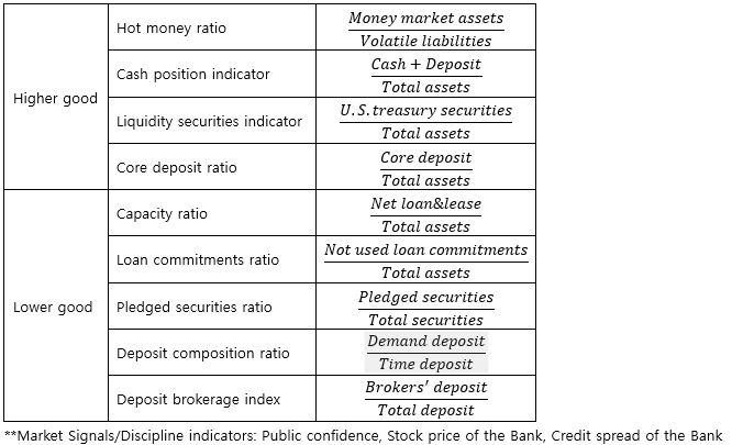
▶Liquidity indicator
▶Types of deposits
|
Demand deposit
|
입/출금
|
이자
|
||
|
Non-interest bearing
|
O
|
X
|
||
|
Interest bearing (NOW)
|
Prior notice 필요
|
O
|
||
|
Money market deposit (Super NOW)
|
O
|
O
(시장 이자율)
|
||
|
Mobile check
|
인터넷 뱅킹 상용화로 실용성 의문
|
O
|
O
|
|
|
Non-transaction deposit
|
입/출금
|
이자
|
||
|
Passbook
|
수시 출금 가능
|
O
|
O
|
|
|
CDs
|
Bump-up
|
더 높은 이자율로 교체 가능
|
X
|
O
|
|
Step-up
|
이자율 주기적으로 상승
|
X
|
O
|
|
|
Liquid
|
약간의 인출 가능
|
O
|
O
|
|
|
Index
|
기초 자산과 연계
|
X
|
O
|
|
**Regulation Q: Demand deposit 이자 지급 제한, Saving deposit에도 한정된 이자만 지급하도록 함
→ 과도한 이자 경쟁으로인한 은행의 건전성 악화 방지
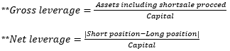
▶Margin loan/Shortsale
|
Margin loan
|
|||
|
Asset
|
Liabilities/Equity
|
||
|
-
|
-
|
-
|
-
|
|
Cash
|
200
|
Equity
|
200
|
|
↓
(Stock 200의 Haircut=50% 따라서 Margin loan 100 가능)
|
|||
|
Asset
|
Liabilities/Equity
|
||
|
Stock
|
200
|
Margin loan
|
100
|
|
-
|
-
|
Equity
|
100
|
|
↓
|
|||
|
Asset
|
Liabilities/Equity
|
||
|
Stock
|
200
|
Margin loan
|
100
|
|
Cash
|
100
|
Equity
|
200
|
|
Shortsale
|
|||
|
Asset
|
Liabilities/Equity
|
||
|
-
|
-
|
-
|
-
|
|
Cash
|
200
|
Equity
|
200
|
|
↓
(Stock 200의 공매도 증거금 50% 따라서 Margin 100)
|
|||
|
Asset
|
Liabilities/Equity
|
||
|
Margin
|
100
|
Borrowed stock
|
200
|
|
Shortsale proceed
|
200
|
Equity
|
100
|
|
↓
Due from broker=Margin+Shortsale proceed
|
|||
|
Asset
|
Liabilities/Equity
|
||
|
Due from broker
|
300
|
Borrowed stock
|
200
|
|
Cash
|
100
|
Equity
|
200
|
▶파생상품의 Balancesheet 반영
|
Future/Forward/Swap
|
Market value of underlying asset
|
|
Option
|
Market value of underlying asset*Option's delta
|
|
TRS
|
기초 자산 Shortsale로 반영
|
|
CDS 판매 (매도)
|
FRN 매수로 반영
|
|
파생상품 Balancesheet
|
|||
|
Asset
|
Liabilities/Equity
|
||
|
-
|
-
|
-
|
-
|
|
Cash
|
100
|
Equity
|
100
|
|
↓
1. $100 Currency forward contract → $100 Asset/$100 Short-term loan
2. $100 Price stock ATM Call option 매수 → $50 Call option/$50 Short-term loan
3. $100 TRS 매수 → $150 ($100 Proceed+$50 Margin)/$100 Borrowed stock
4. $100 CDS 매도 → $100 FRN 매수/$100 Term-loan
|
|||
|
Asset
|
Liabilities/Equity
|
||
|
1. Currency forward
|
100
|
Short-term loan
|
100
|
|
2. Call option
|
50
|
Short-term loan
|
50
|
|
3. TRS
|
|
|
|
|
Proceed
|
100
|
Borrowed stock
|
100
|
|
Margin
|
50
|
|
|
|
4. CDS 판매
|
|
|
|
|
FRN 매수
|
100
|
Term-loan
|
100
|
|
Cash
(Margin으로 50 사용)
|
50
|
Equity
|
100
|
▶EWI guidelines
|
OCC
|
Consider embedded options
|
|
BCBS (2012)
|
Consider intraday liquidity
|
▶Incorporate liquidity risk to VaR
|
Exogenous (외부요인)
|
Bid/Ask spread → Liquidity VaR로 거래 비용 반영
|
|
Endogenous (내부요인)
|
해당 회사가 많은 양을 거래하며 생기는 불리한 시장 충격 → 반영하기 어려움
|
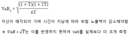
▶Liquidity adjusted VaR
▶Source of Transaction risk
|
Trade process cost
|
거래 상대방을 찾는 비용, 거래 인프라에 문제가 없는 경우 Liquidity risk를 가중시키지 않음
|
|
Inventory management
|
Dealer는 거래의 즉시성을 위해 Short/Long 자산을 보유
→ 변동성 위험에 노출
|
|
Adverse selection
|
Dealer는 거래 상대방에 대한 정보 부족
Bid-Ask spread를 통해 보상을 받음
|
|
Differences of opinion
|
Agreed Market의 경우 거래 상대방을 찾기 힘듦
|
|
Slippage
|
주문 후 거래가 체결되기 전까지의 시간으로 생기는 손실
|
|
Quote-driven
|
Market maker가 호가 제시 (OTC에서 주로 사용)
|
|
Order-driven
|
Competitive auction model
|
▶Legal liquidity reserve calculation
Day 01(화) ~ Day 14(월) → Reserve computation period (13-Days)
Day 15(화) ~ Day 30(수) → Planning period (15-Days)
Day 31(목) ~ Day 44(수) → Reserve maintenance period (13-Days)
▶Liquidity option
|
Financial option
|
Profitability에 따라 행사 결정 (Independent of Cashflow)
|
|
Liquidity option
|
Cashflow에 따라 행사 결정 (Independent of Profitability)
|
▶Dealer bank risk
|
High leverage
|
Lack of capital requirements especially to off-balance assets
|
|
Diseconomies of scope
|
규모가 너무 커져 리스크 관리가 어려워짐
|
**U.K.: 고객의 자산을 딜러 뱅크의 자산과 혼합/U.S.: 고객의 자산을 딜러 뱅크 자산과 분리
▶Intraday liquidity
대부분 Wire transfer에 대응하기 위해 필요 (Retail의 경우 고객들의 행동을 예측하기 어려움)
|
PCS (지불청산시스템)
|
Single-day payment는 Multi-day payment 보다 예측하기 어려움
|
|
Securities/Fixed asset purchase
|
거래 후 2영업일 이후 결제 (예측성 높음)
|
|
Client loan
|
예측이 어려움
|
|
Tracking
|
Monitoring
|
||
|
Total payments&Other transactions
|
Daily maximum usage
(Not require real-time data)
|
Most negative balance
|
|
|
Settlement position
|
결제 Deadline/Amounts
|
Intraday credit to T1 capital
(Capture Systemic risk)
|
Unsecured&Available credit/Tier 1 capital
|
|
Time sensitive
Obligations
|
Late settlements
→ Penalty
Deadline 관리 필요
|
Payment throughput
(Trading Patterns)
|
분포를 통해 Outflow가 많은 시간대 예측
|
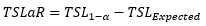
▶Term structure of liquidity (TSL)
|
Expected cash flow
|
Customer behavior, Default/Correlation 등을 기댓값을 통해 예측
(Stochastic CF)
|
|
Balancesheet expansion
|
차입, 채권 발행 등을 통해 자금 확보
|
|
Balancesheet shrinkage
|
자산을 매각해 자금 확보
|
**Possession: 역레포 시 상대의 자산을 보유/Ownership: 레포 시 상대에게 자산을 넘기지만 소유권은 유지
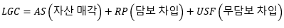
AS, RP는 Balance sheet → Reduce/Constant
USF는 Balance sheet → Expansion
▶TARP Program
금융 위기 이후 Dealer bank가 자금 보충을 위해 낮은 가격으로 자산을 매각해야 했음 (Adverse selection)
→ Dealer bank의 손실이 더욱 커질 위험
1. TARP 프로그램을 통해 부실 자산을 매수해 Dealer bank의 손실을 흡수 (Beyond predetermined level)
2. 시장보다 더 낮은 수준의 금리를 적용해 자금을 공급
▶Stressed liquidity buffer (Contigent liquidity)
Stressed liquidity buffer=Normal liquidity buffer+(Stressed cash inflow-Stressed cash outflow)
Stressed cash outflow: Early settlement, Failure of Rollover, Decrease in Funding source
▶Liquidity stresstest
1. Foreign entities: Separate stresstest
2. Lack of empirical data: Historical stresstest보다 다양한 가정으로 Hypothetical stresstest 시행
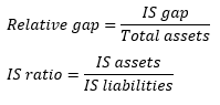
▶Relative gap/Interest sensitivity ratio
▶Contigency funding plan
|
Governance
|
Corporate treasury
|
Oversight, Involved in LCT
|
|
|
Liquidity crisis team (LCT)
|
Monitoring/Communication
Executives, Business unit leaders, Senior managers로 구성
|
||
|
Management committee
|
Manage/Oversight LCT
|
||
|
Monitoring/
Escalation
|
EWI
|
Macro/Micro/Liquidity health measure
|
|
|
Escalation
Level
|
Level 1
|
Oversight/Monitoring/Communication
|
|
|
Level 2
|
Events occur and clearly negatively impacting to firm
Analyzing the causes
|
||
|
Level 3
|
Executing/Undertaking activities to survive
|
||
▶Reasons of global financial crisis
1. Decentralized liquidity management: Not updated frequently, Internal arbitrage
2. Zero-cost approach: 장기/비유동 자산의 위험을 제대로 인지하지 못함
3. Increase of USD assets: Off-balance vehicle의 Balancesheet 편입 → Dollar shortage
4. Hard to sell complex securitization products (CDO)
→ 금융 위기 당시 Funding gap은 583 Billion으로 측정되었지만 이는 Write-down (평가절하)에 의해 과소평가된 것 실제로는 880 Billion로 추정
**Fed’s Reciprocal swap arrangement (Local 통화를 담보로 USD 공급) → Lender of last resort
1. Fed는 USD를 무제한으로 제공할 수 있으므로 안정성이 높음
2. Local 통화를 담보로 하므로 Moral hazard 문제가 적음
▶Limitations to IS/Duration gap
|
IS gap
|
이자율의 변화가 모든 자산/부채에 동일하게 반영되지 않음
Ex) 이자율 상승 시 Deposit의 이자율은 천천히, Loan의 이자율은 빠르게 반영
→ Weighted IS gap을 통해 완화 가능
Repricing을 포착하기 어려움
|
|
Duration gap
|
Duration 측정의 어려움 (Cash-flow를 예측하기 어려움)
이자율의 Small change에만 사용 가능 (Convexity 고려 불가)
Parallel change to yield curve 가정
|
▶Foreign Exchange (FX) swaps/Cross-currency basis swaps
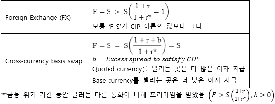
CIP 위배의 요인
1. Lack of liquidity: Wider Bid-Ask spread/Transcation cost → Arbitrage 거래가 비활성화
2. Risk premia to counterparty risk: 약간의 Premia에도 Hedge demand가 큼 → Arbitrage 거래가 비활성화
**Risk premia: FX market (LIBOR-OIS로 측정), Sovereign (CDS spread로 측정)
▶BA/SA Operational risk capital requirement
Business indicator (BI)
|
BIC Weight
|
Business
|
|
12%
|
Retail, Asset management
|
|
15%
|
Commercial, Agency
|
|
18%
|
IB (Corporate finance), Payment&Settlement, Trading
|
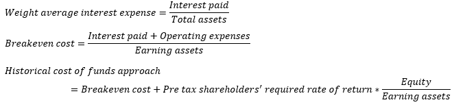
▶Cost of funds – Pooled funds approach
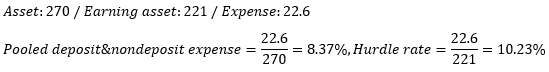
▶Cost of funds – Historical cost of funds approach
▶Liquidity risks
|
Transaction risk
|
자산 매각 과정에서 비우호적인 가격 움직임 발생
|
|
Funding risk (Balance sheet risk)
|
자산과 부채의 만기 불일치로 인한 유동성/롤 오버 리스크
|
▶Deterministic and Stochastic cash flows
|
Cash flows
|
Time
|
||
|
Deterministic
|
Stochastic
|
||
|
Amount
|
Deterministic
|
Fixed-rate coupons bond
|
Withdrawals from credit lines
(Amount limits)
|
|
Stochastic
|
European option
Floating-rate coupons bond
Bank issues new debt
Contract renewals
|
American option
Demand deposit withdrawals
New loans
|
|
▶Contributor to U.S. dollar shortage
1. Drawn of credit commitments
2. Structured products (CDO) became more difficult to sell
3. Banks brought off-balance vehicles back to their balance sheet
▶EWI
▶Illiquid asset bias
|
Bias
|
Return
|
Risk
|
|
|
Survivorship bias
|
수익률이 높은 펀드만 보고 (Reporting bias)
수익률이 나쁜 펀드는 결국 사라짐 (Survivorship bias)
|
↑
(Return)
|
|
|
Selection bias
|
높은 가격에서만 거래가 되는 경우가 많은 경우
→ Buyout/Venture capital/Distressed strategy funds
|
↑
(α)
|
↓
(β, σ)
|
|
Infrequent trading
|
Understate risk
|
|
↓
(β, σ, ρ)
|
|
Smoothed data
|
Overstate return, Understate risk
→ Filtering algorithm: Noise를 추가하여 Smoothed data 효과를 감소
|
↑
(Return)
|
↓
(α)
|
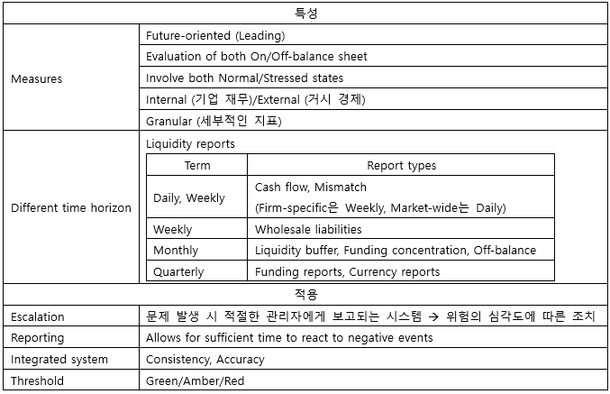
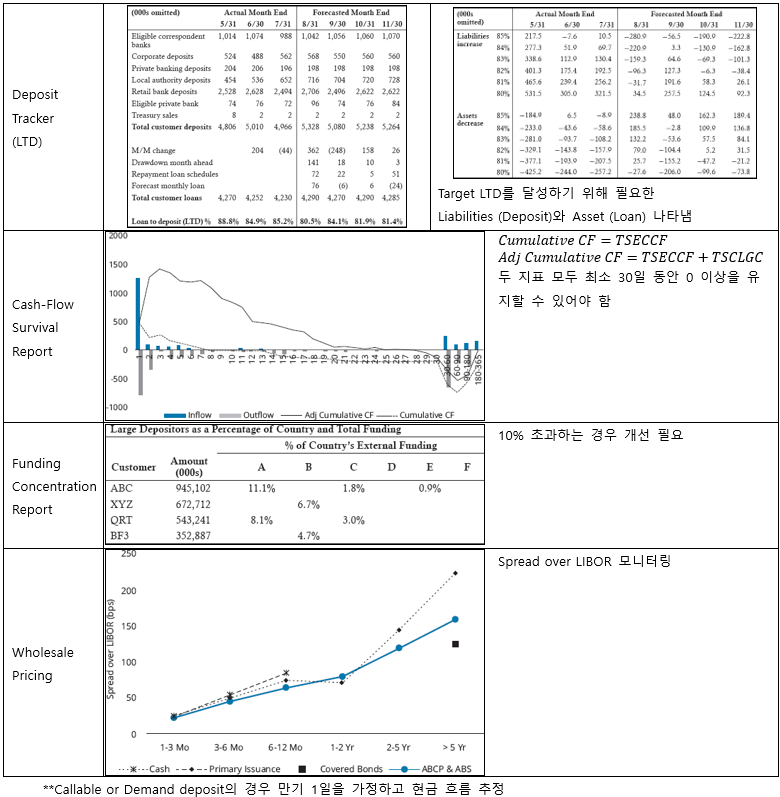
▶Liquidity reports
▶Illiquid effects
|
U.S. treasury market
|
Yield of Off-the-run > Yield of On-the-run
|
|
Corporate bond market
|
Larger bid-ask spread/Infrequent traded bonds → Higher yield
|
|
Equity market
|
High bid-ask spread
Low volume
Low turnover
Infrequent trades
Many numbers of zero returns
|
▶Harvest of illiquidity premium
|
Passive allocation
|
포트폴리오에 비유동적 자산 추가
|
|
|
Liquidity security selection
|
자산군 내에서 종목 선택 시 비유동적 자산 선택
→ 소형주>대형주, Off-the-run>On-the-run
|
|
|
Market maker
|
Dealer, 비유동적 자산을 싸게 매입한 뒤 수요자를 찾아 매도
|
|
|
Dynamic factor strategy
|
Arbitrage
|
유동적 자산 매도, 비유동적 자산 매수로 차익 거래
|
|
Rebalancing
|
비유동적 시기에 자산을 매수, 유동적 시기에 자산 매도
(Countercyclical)
→ Easiest and Great impact
|
|
▶Cost of deposit
|
Cost-plus
|
Operating expense+Overhead cost+Required margin
|
|
|
Marginal cost
|
ΔCost/ΔDeposit
|
|
|
Conditional pricing
|
Flat rate
|
서비스 이용시 일정한 비용 부과
|
|
Free pricing
|
무료 (실제로는 고객의 기회 비용 발생)
|
|
|
Conditionally Free
|
큰 금액의 계좌는 무료, 작은 금액의 계좌는 요금 부과
|
|
|
Relationship pricing
|
고객이 다른 서비스를 이용하는 여부에 따라 요금이 달라짐
|
|
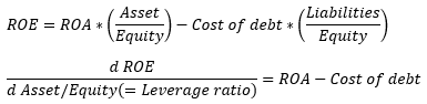
▶ROE/ROA
Chapter 5
Risk management and investment management
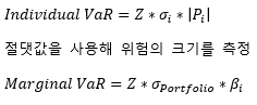
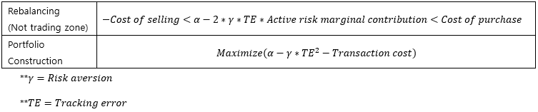
▶Marginal VaR & Portfolio construction
▶Value vs Growth vs Momentum
|
Value
|
Growth
|
Momentum
|
|
Value 주식이 더 높은 수익률을 보이는 이유
Rational:
Value 주식의 Asymmetric/High Adjustment cost → More risky
Behavioral:
투자자들이 Growth 주식을 고평가하여 낮은 수익률을 가짐
Value premium:
Hard to seek/Long investment horizon
→ Size factor와 다르게 쉽게 사라지지 않음
|
Over/Underreaction → Momentum
Inherent destabilizing (Positive feedback)
Risks:
1. Tendency toward crahses (폭락)
2. 정부/통화 정책의 개입 리스크
|
|
**Value premium과 Momentum premium이 강한 Negative relationship을 가지진 않음 (-0.16, During 2007-2009)
▶Types of value investing
|
Bond
|
Commodity
|
Currency
|
|
Riding the yield curve
|
Roll return
|
Carry:
높은 이자율의 통화에 Long
낮은 이자율의 통화에 Short
|
▶Risk aversion
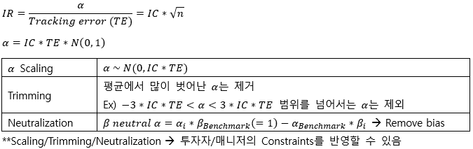
▶Sharpe/IR ratio
|
(+)
|
Easy to compare with peer
Apply to industrial sectors and countries
|
|
(-)
|
Not forward looking
Insufficient data available to perform calculations
|
▶Benchmarking a portfolio
벤치마크와 같은 듀레이션으로 포트폴리오를 구성해도 Non-parallel shift로 인해 Tracking error 발생
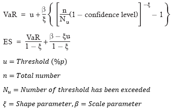
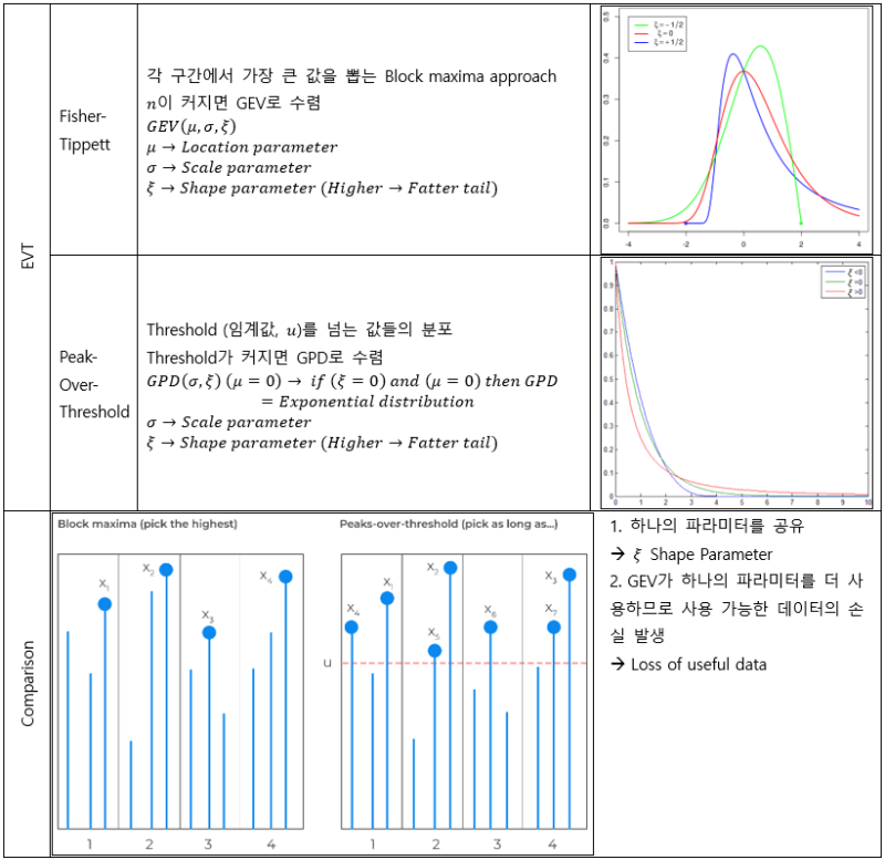
▶POT(GPD) Model VaR/ES
▶Marginal VaR
▶GEV/GPD
▶Portfolio construction
|
Quadratic
|
Mean-variance, 마코위츠 포트폴리오 → 많은 계산을 통해 Optimal portfolio 구축
(Alphas, Risks, Transaction costs, Pair-wise correlation 등을 고려)
Too many calibrations, Potential for noise (Estimation error)
|
|
Screening
|
특정 기준을 만족하는 Stocks 선별 → 충분한 수의 종목/비중 조절
But can ignore entire sectors or classes of stocks if they do not pass the screen
|
|
Stratification
|
포트폴리오의 Sector weights를 Benchmark와 동일하게 조절 (배타적 Categories)
|
|
Linear programming
|
Stratification보다 더 많은 Dimension을 고려하는 방법 하지만 배타적이진 않음
|
▶α scaling/β neutral α
▶Portfolio construction
▶Transaction cost
|
Transaction cost
|
Occur at points in time, 보유 자산의 Holding period가 불확실
→ Having difficulty in what period transaction cost should be amortized
|
|
Benefits of trading
|
Realized over time
|
▶Correct illiquid asset bias
|
Low volatility
|
Positive ACFs, Long horizon 추정을 통해 완화
|
|
Low correlation
|
Use regression with additional lags of the market factors and sum the coefficients across lags
|
▶Dispersion
Dispersion: 같은 Portfolio 내에서 각 고객들 간의 수익률 차이
새로운 고객의 계좌를 기존 고객과 일치시켜 Dispersion 해결 → 새로운 최적 분배 비율의 편익 포기
빈번한 리밸런싱으로 Dispersion 해결 → 과도한 거래비용
|
요인
|
Client-driven
|
고객의 투자 제약 (특정 상품 편입 불가)
|
|
Management-driven
|
포트폴리오 매니저의 부주의
|
|
|
외부요인
|
거래 비용
|
|
|
Dispersion은 Number of portfolio/Active risk가 커질수록 증가
|
||
|
Not Constant /Risk → Dispersion은 천천히 감소하며 수렴 (어느 Level로 수렴하는지는 모름)
|
||
|
Dual-Benchmark
|
Dispersion은 완화되지만 Average return 감소
|
|
▶Assumptions of CAPM
|
Only have Financial wealth
|
In real world, investors have many factors that contribute to wealth
Ex) Human capital
|
|
Mean-Variance utility
|
Assumes a symmetric treatment of risk
In real world, investors dislikng losses more than they like gains
**Infinitely risk-averse (X)/Infinitely risk-tolerant (O)
Infinitely risk-averse (X) → Risk-free 자산만 보유하고 있는 투자자는 없다고 가정
|
|
Single-period horizon
|
CAPM assumes single-period investment horizon → No rebalancing
In real world, investors have multi-period strategy
|
|
Information is free (costless) and available to everyone
|
|
|
Risk premiums will not disappear since investors cannot use arbitrage to remove systematic risk
|
|
**CAPM, Fama-French model → β가 Constant하다고 가정, 하지만 현실에서는 Bad time에 β 증가
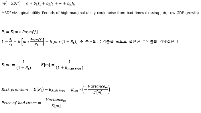
▶Expected payoff in bad times and expected return
|
Low expected payoff in bad times
|
→
|
High β
|
→
|
High expected return
|
|
High expected payoff in bad times
|
→
|
Low β
|
→
|
Low expected return
|
▶Pricing Kernels (Stochastic discount factor)
▶Efficient market theory
|
APT
|
Uses systematic factors that cannot be removed through arbitrage
→ Premium으로 보상 받음
(CAPM과 비슷한 가정)
|
|
Sanford Grossman and Joseph Stiglitz Theory
|
Markets are near efficient and information is costless
모순: 정보 비용이 없고 가격이 모든 정보를 이미 반영하고 있다면 시장 참여자들이 정보 획득에 노력할 이유가 없음 → 하지만, 누구도 정보를 모으지 않는다면 효율적 시장이 될 수 없음
|
|
Efficient market hypothesis (EMH)
|
Implies that speculative trading is costly, and active managers cannot beat the market
비효율성 인정 (Imperfect information, Various costs, Behavioral biases)
Rational explanation: Losses during bad times are compensated by high returns
→ 하지만, Bad time은 각자 사람마다 다를 수 있음 (Short market 투자자는 Bad time에 수익)
Behavioral explanation: 투자자들의 Over/Underreaction → Inefficiency
|
▶Characteristic of appropriate benchmark
1. Well-defined
2. Tradeable
3. Replicable
▶Investment returns during expansions and recessions
|
|
Stock
|
Government Bonds
|
Corporate Bonds
|
|
|
Investment Grade
|
High Yield bonds (경기의 영향이 적음)
|
|||
|
Expansion Business cycle
|
↑
|
↓
|
↓
|
↑(작은 폭)
|
|
High GDP growth
|
↑
|
↓
|
↓
|
↑(작은 폭)
|
|
High Consumption
|
↑
|
↓
|
↓
|
↑(작은 폭)
|
|
High Inflation
|
↓
|
↓
|
↓
|
↓
|
**주식은 실물 자산에 대한 소유권을 나타내므로 High inflation에서의 Poor perform이 불명확
**Government bonds/Investment grade bonds는 안전 자산의 특성을 보여줌
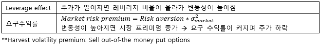
▶Volatility and stock return
변동성은 주식 수익률과 Negative relationship을 가짐
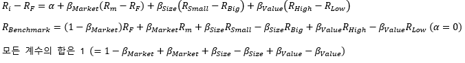
▶CAPM regression
▶Active risk
Active management risk is not much of a problem
1. For Well-managed funds, it is usually fairly small for each of the individual funds
2. Diversification effects
3. Diversification effects with policy mix VaR → Lower total portfolio VaR
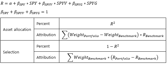
▶Style analysis
Factor를 Tradeable 자산으로 대체 (SPY: S&P500 ETF, SPYV: S&P500 가치주 ETF, SPYG: S&P500 성장주 ETF)
▶Anomalies
|
Low-risk anomaly
|
Lower β/σ → Higher Return (Violation of CAPM)
|
|
Volatility anomaly
|
Lower σ → Higher Return/Sharpe ratio
|
|
Beta anomaly
|
Lower β → Higher Sharpe ratio
|
→ CAPM은 Lagged beta (후행적 Metrics)를 사용하므로 예측력 떨어짐, 투자 기간과 동일한 기간을 지닌 β 필요
→ Implied volatility를 이용해 Future β를 추정하려는 시도 존재
Possible explanations:
1. Leverage 사용이 어려운 투자자들은 High β에 투자하는 경향 존재 → High β 종목의 가격↑/수익률↓
2. Constraints to Short sale/Tracking error for institutional managers
3. 투자자들이 높은 변동성 종목을 선호함 → High β 종목의 가격↑/수익률↓
▶Portable α Strategy
β=0 인 상태로 Positive α를 만들어 시장 상황에 관계없이 수익을 얻는 전략
1. Hedge funds 전략의 위험들은 Non-linear인 경우가 많아 평가하기 어려움
2. Hedge funds의 보유 자산이 비유동적인 경우가 많음
3. Hedge funds 전략은 Market crisis에 민감한 경우가 많음
→ 이러한 이유들로 위험을 정확히 평가하기 어려움
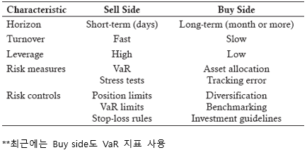
▶Sell side/Buy side
▶Weight of portfolio managed by manager

▶Risk planning/budgeting/monitoring
|
Risk Planning
|
수익률/변동성 목표 설정, ROE/RORC를 활용해 성공/실패 기준 설정
|
|
Risk Budgeting
(Top-down)
|
ROE/RORC/Mean-variance/Simulation 활용해 Risk capital 할당
Weights를 바탕으로 성과 Simulate
Sensitivity analysis를 통해 추정치의 변화가 성과에 주는 영향 분석
|
|
Risk Monitoring
|
Monitoring → Risk management unit (RMU)
RMU는 Gathering/Monitoring/Analyzing/Distribution 수행
|
▶Use of VaR
|
Catch rogue trader
|
||
|
Detect changes in risk
|
||
|
Traditional vs VaR
|
Traditional
|
Notional (명목 금액) Limit에 집중, Not overall risk
|
|
VaR
|
Relying less on notionals, Focusing more on overall risk
|
|
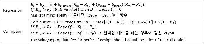
▶Measuring market timing
▶Failure of funds
1. Poor investment decisions
2. Fraud/Poor internal controls
3. Leverage
4. Lack of liquidity
5. Insufficient questioning: Committee-style → Dominant member의 영향력 과다 (Devil’s advocate로 완화)
6. Insufficient attention to returns: Risk 관리에만 몰두하여 수익률이 너무 낮아짐
▶Fund manager evaluations
1. Strategy
2. Ownership: Manager’s interests aligned with investor’s interests
3. Track record: Past performance → 하지만, 과거 성과에 너무 의존하면 안 됨
4. Investment management:
Reference checks: Former employers, Colleagues, Investors
Background checks: Form ADV (규모 25 Million 이상)
**이전의 SEC는 가장 최근의 Form ADV만 제공했지만 투명성을 개선하기 위해 과거 데이터도 제공하며 표준화된 형식을 지니게 됨
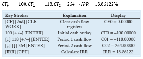
▶Dollar-weighted rate of return (IRR)
▶Time-weighted rate of return
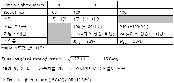
▶IRR VS Time-weighted return
|
IRR
|
Poor portfolio performance → IRR tend to be depressed
Favorable time → IRR will increase
매니저가 Money flow에 Control을 가지고 있는 경우 IRR이 더 적합함
(If manager has superior market timing ability → IRR>Time-weighted return)
|
|
Time-weighted return
|
Only capture manager’s ability
|
▶Hedge fund strategies
|
Managed futures
|
High leverage, Market timing
(Similar to a lookback straddle)
|
Trend following
Asset allocation
Low correlation
|
|
|
Global macro
|
Directional movements (Long/Short)
|
||
|
Merger/Distressed
|
Short put option과 비슷한 수익 구조로 극단적 상황에서 큰 손실 발생 (Tail risk)
Non-linear, Event driven, Distressed securities strategy≒Buy High-yield bonds
|
||
|
Fixed income
Arbitrage
|
Swap spread
|
Fixed payment와 Floating payment의 Spread로 차익거래
|
|
|
Yield curve
|
채권 가격의 일시적 Deviate 포착
|
||
|
Mortgage Spread
|
Prepayment rate로 차익거래
|
||
|
Fixed income Volatility
|
내재변동성과 실현변동성 차이로 차익거래
|
||
|
Capital structure/
Credit arbitrage
|
다른 상품 간 Mispricing 포착
|
||
|
Emerging markets
|
Short 거래가 어려워 Long bias 존재
|
||
|
Equity Long/Short
|
유동성 위기를 대비해 Liquidity buffer 설정 필요
|
||
**2000년대 초부터 기관 투자자의 자금이 많이 유입 (S&P 500 대비 헤지펀드 인덱스의 수익률, 위험 모두 우월)
**2002-2010년까지 α가 지속적으로 감소 (헤지펀드 시장의 경쟁 심화, Hard to seek α)
**Top 50 hedge funds outperformed hedge fund indices
▶Factors that affect to funds fraud
|
Conflicts of interest
|
Significantly Related to fraud
|
|
|
The broker/dealer
|
회사가 브로커/딜러와 많이 연관될수록 사기의 위험이 커짐
|
|
|
Registration ICA
|
더 높은 규제 적용 → 사기 위험 감소
|
|
|
Investor size
|
작은 규모일수록 사기의 위험이 큼
|
|
|
Clients who are agents
|
Like a pension fund manager who is the client but not a direct beneficiary of the funds (대리인이 고객인 경우)
|
|
|
Soft dollar
|
브로커에게서 리베이트를 수취하며 거래를 맡김
|
Not significantly Related to fraud
|
|
Custodian
|
Custodian은 사기의 위험이 더 클 수 있음
|
|
|
Employee owned
(Internally owned)
|
Externally owned 회사에 비해 감시가 부족
|
|
|
Chief compliance officer (CCO)
|
CCO가 존재하는 것이 사기 감소에 직접적 영향을 주진 않음
|
|
|
Manage hedge funds
|
헤지펀드의 불투명성이 사기에 영향을 줄 수 있음
|
|
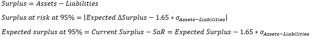
▶Surplus at risk
Chapter 6
Current issues in financial markets
▶Phillips curve
|
Simplicity
|
Constant relationship 가정
Low-inflation 환경에서만 잘 맞음
|
|
Aggregate price index
|
Sectoral 영향보다 전체적 영향 고려
|
|
Cyclical factors
|
Aggregate demand 측면
(↔ Structural factors: Pricing power of Labors, Wage-Price spiral)
|
▶Inflation
|
|
Low inflation
|
High inflation
|
|
Sensitivity to inflaiton
|
Low
|
High
|
|
Wage-Price spiral
|
Low
|
High
|
|
Stability
|
Self-stabilization
|
Not Self-stabilization
|
|
Correlation
|
각 상품 가격의 상관성이 낮음
|
각 상품 가격의 상관성이 높아짐
|
**낮은 인플레이션은 낮은 가격 변동성 때문이 아닌 낮은 상관성에 의한 것
▶Inflation expectation channels
|
Interest rate
|
높은 인플레이션이 예상되면 더 높은 수익률을 요구 → 명목 이자율 상승
|
|
|
Exchange rate
|
높은 인플레이션이 예상되면 자본이 유출 → 통화 평가절하
|
|
|
Financial market
|
옵션 가격을 이용해 미래 인플레이션 예상
→ 다른 요인들도 가격에 영향을 주므로 인플레이션만의 영향을 제대로 파악하기 어려움
|
|
|
Household/
Financial market
|
Household
|
인플레이션을 과대 평가, 후행적
|
|
Financial market
|
정확도 높음
|
|
▶Transition to High inflation
|
Core inflation index
|
변동성이 높은 식료품/에너지 가격을 제외해 추세의 변화 파악 용이
|
|
Second-round effects
|
가격 변화에 따른 임금의 변화를 측정
|
|
Wage indexation abandon
|
물가 연동보다 더 높은 임금상승률 요구
|
|
Centralized bargaining
|
노동 조합 등의 임금 협상력 증가
|
|
Weak public finance
|
|
▶Use of AI
|
Credit risk
|
Decision Tree, SVM
|
|
Market risk
|
Reinforcement learning
|
|
Operational risk
|
Automated system (Human error 감소)
|
|
Regulatory compliance
|
NLP, RegTech
|
▶AI Risk
|
Data
|
Learning limitation
Data quality
|
|
|
AI/ML Attack
|
Data privacy attack
|
Differential privacy로 완화 → 노이즈를 추가해 익명성 유지
|
|
Data poisoning
|
Training data의 오염으로 Errorneous output 산출
|
|
|
Adversarial input
|
Misclassification 유도
|
|
|
Model extraction
|
모델 탈취 → Most serious type of attack
Watermarking으로 완화
→ 특정값 입력 시 특정값이 산출되도록 하여 탈취한 모델임을 확인 가능
|
|
|
Membership inference
|
Output을 통해 내부 데이터 추론
|
|
|
Discrimination
|
Manual approach 필요 (AI 시스템 보완)
Minimizing disparate: 차별적 변수들 제거
Mitigation algorithm: 동일한 차별 정도에서 가장 적합한 모델 선택
|
|
|
Explainability
|
같은 결과에도 다른 설명 가능 (Inconsistent explanation)
스스로 학습하는 특성으로 Output이 일정하지 않아 검증이 어려움
Black box problem (Lack of transparency)
|
|
▶AI risk mitigation
1. AI의 Process/Methods 이해
2. Review data quality
3. Accuracy drift monitoring: Accuracy의 감소를 빠르게 파악
4. Data drift monitoring: Training data와 Input data의 괴리를 빠르게 파악
|
Pre-processing approach
|
AI 알고리즘 내의 Decision-making 과정을 파악
|
|
Post-processing approach
|
도출된 Out-put을 분석 (Black box approach) → 대부분의 방식에 사용 가능
|
▶Climate risk
1. Credit/Market risk에 주로 영향을 미침
2. Transition risk>Physical risk
3. Concentration risk 중요
▶Climate risk challenges
|
Capture economic effects
|
Chronic risk
|
Can be modeled
|
|
Acute risk
|
Hard to modeled
|
|
|
Long-term horizon
|
5-Year 이상으로 분석되어야 하므로 더 큰 Complexity
|
|
|
Operational assessment
|
Proper IT System/전문인력 양성 비용 多
Out-sourcing cost 多
|
|
▶Granularity
|
Higher granularity
|
High complexity, Suffer from input data, More valuable for valuations
|
|
Lower granularity
|
Better suited to portfolio allocations and strategic planning
Less complexity, More tolerant of sporadic data
|
▶Sectors that influenced by physical/transition risks
|
Risk types
|
Sectors
|
|
|
Physical
|
Utilies
|
Agriculture, Real estate (Retail mortgages)
|
|
Transition
|
Energy/Oil/Gas, Transportation, Construction
|
|
▶Challenges to comparability of climate risks
1. Cross-jurisdictional standards is a challenge (Jurisdictional difference)
2. Group-wide policy may conflict with climate risks unique to location (Geographic difference)
3. Lack of data quality:
Lack of Granularity/Not-Frequent updates
Third-party data 사용 시 데이터의 출처와 정확성 정보 부족/각 제공자 사이의 Standard가 확립되지 않음
Banks may not be able to easily update data after underwriting processes have concluded
▶Climate risk mitigation
|
Scenario test
|
Transition risk test
|
Long/Short horizon
|
|
Physical risk test
|
Long horizon
|
|
|
Not front-loaded
|
데이터 부족, 정립된 위험 관리가 없으므로 계속적으로 수정해나가는 방식으로 발전
(Iteratively, Progressively, As-needed basis approach)
|
|
|
위험 분산
|
Systematic/Extreme risk에는 취약
|
|
|
Insurance
|
Insurance cover rate가 낮아지는 문제
|
|
|
Catastrophe bond
|
Trigger event 발생 시 투자자 손실 발생 → 위험 이전 효과
금액이 아닌 사건 발생을 기준으로 Trigger
|
|
|
Weather derivatives
|
Local 위험 관리에 효율적이지만 Global 위험 관리는 어려움
→ 하지만, 최근의 ESG Future, Carbon derivatives는 Global 위험 관리에 사용 가능
|
|
▶Climate risk measure methods
|
IAM (Integrated assessment model)
|
Combine economic, energy, climate modeling
Can’t capture extreme weather (Underestimate severe events)
|
|
|
Input-Output model
|
Capture policy shift impact
|
|
|
General
Equilibrium
|
Computable
|
Capture complex interactions → 많은 계산량
|
|
Dynamic stochastic
|
||
|
Overlapping generation model
|
Capture Long-term macroeconomic factors
|
|
|
Agent-based model
|
Complex, High flexibility, Need large amount of computation
|
|
|
Scenario
Analysis
|
Scenario analysis
|
Physical/Transition scenario analysis
|
|
Sensitive analysis
|
Capture policy shift impact (특정 변수가 미치는 영향 분석)
Underestimate tail events
|
|
|
Natural capital analysis
|
천연 자원의 감소가 미치는 영향 분석 (3rd Party approach)
|
|
|
Climate VaR
|
Climate risk가 Balancesheet에 미치는 영향 분석 (3rd Party approach)
|
|
|
Climate risk rating
|
내부/외부 Rating
|
|
**Static balance sheet: Current Exposure을 보여줌 → Time horizon이 길어질수록 신뢰도 하락
**Dynamic balance sheet: Exposure에 영향을 주는 Strategy adjustments를 고려
▶Stable coin
|
Asset-backed
|
Intermediary 존재, 중개인이 Backed 자산을 관리/투자
|
|
Algorithmic
|
Intermediary 미존재, 코인의 공급을 자동으로 조절해 Pegging
|
▶Centralized/Decentralized exchange
|
Centralized exchange
(CEX)
|
CEX 데이터 베이스에 거래 기록, Low transaction cost
거래소의 보유 자산이 투명하게 공개되지 않을 위험 (Poor Public disclosure)
|
|
|
Decentralized exchange
(DEX)
|
Peer-to-Peer (On-chain/Off-chain), Smart contract (Offset the risk of possible bank run)
|
|
|
Dex aggregators
|
다수의 DEX가 모여 유동성 확보
|
|
|
AMM
|
이용자들이 자산을 배치하도록 인센티브를 제공해 유동성 확보
Most successful type of DEX
|
|
▶CBDC
|
Wholesale CBDC
|
Smart contract (Atomic settlement)
|
Instantaneously, No human involvement
|
|
Zero-knowledge proofs
|
익명성을 유지하며 사용자 증명 가능
|
|
|
Retail CBDC
|
Retail FPS
|
Private Bank가 중개인
|
|
Retail CBDC
|
Peet-to-Peer/Privacy risk 감소
|
▶Features of the future monetary system
1. Safety and stability: 가치 보존, 거래의 단위, 교환의 매체 → 통화의 역할
2. Accountability: 투명성, 책임
3. Efficiency: Low-cost, Fast transaction
4. Inclusion: 다양한 서비스를 포괄
5. Integrity: Anti money laundering and terrorist activity financing
6. Adaptability: Foster competition and innovation
7. Openness: Cross-border use
▶Scalability trilemma (확장성 트릴레마)
Scalability/Security/Decentralization → 세 가지 목표를 한 번에 모두 달성할 수 없음
Security/Decentralization를 위해 Miner에게 보상을 주고 거래를 블록 체인에 기록/검증하는 역할 부여
→ 적절한 인센티브가 있어야 Miner가 참여하므로 그 수가 제한되어야 함 → Congestion↑ (Scalability↓)
**블록체인의 Interoperability (상호 운용성) 부족은 고질적인 문제
'FRM' 카테고리의 다른 글
| 국제 FRM Part I, II 독학 동차 합격 후기 (0) | 2024.01.05 |
|---|---|
| 국제 FRM Part 1 오답·개념 정리 (3) | 2024.01.04 |
'FRM' Related Articles
more

